Session-7 Statisctical Tests
7.1 Hypothesis Testing:
Hypothesis testing is a fundamental statistical method used to make decisions or draw conclusions about populations based on sample data. It involves two competing hypotheses: the null hypothesis (H0), which represents the status quo or no effect, and the alternative hypothesis (Ha), which suggests there is a significant effect.
Example:
Suppose you want to test if a new drug is more effective than an existing one.
Null Hypothesis H0: The new drug has no significant effect;
Alternate Hypothesis Ha: The new drug is more effective.
You collect data from two groups of patients and analyze it to determine if there’s enough evidence to reject the null hypothesis in favor of the alternative.
# Example: Testing the effectiveness of a new drug
# Null hypothesis (H0): The new drug has no significant effect (mean_effect = 0).
# Alternative hypothesis (Ha): The new drug is more effective (mean_effect > 0).

# Generate data for two groups (existing drug and new drug)
set.seed(123)
existing_drug <-  rnorm(30, mean = 75, sd = 10)  # Sample data for existing drug group
new_drug <-  rnorm(30, mean = 80, sd = 10)      # Sample data for new drug group

# Perform a one- sample t- test to compare the new drug group mean to the expected mean (0)
t_result <-  t.test(new_drug, mu = 0, alternative = "greater")

# Print the test result
print(t_result)
##
## One Sample t-test
##
## data: new_drug
## t = 54, df = 29, p-value <2e-16
## alternative hypothesis: true mean is greater than 0
## 95 percent confidence interval:
## 79.19 Inf
## sample estimates:
## mean of x
## 81.78Here as p- value is less than 0.05 (Standard aplha used generally) we REJECT the null hypothesis
# Degrees of freedom (df)
df <- 29 # Degrees of freedom for the one- sample t- test
# Sequence of x- axis values
x <- seq(- 3, 3, by = 0.01) # Adjust the range and step as needed
# Calculate the PDF of the t- distribution
pdf_values <- dt(x, df)
# Plot the t- distribution
plot(x, pdf_values, type = "l", lty = 1, col = "blue",
xlab = "X- axis", ylab = "Probability Density",
main = "t- Distribution for New Drug Group")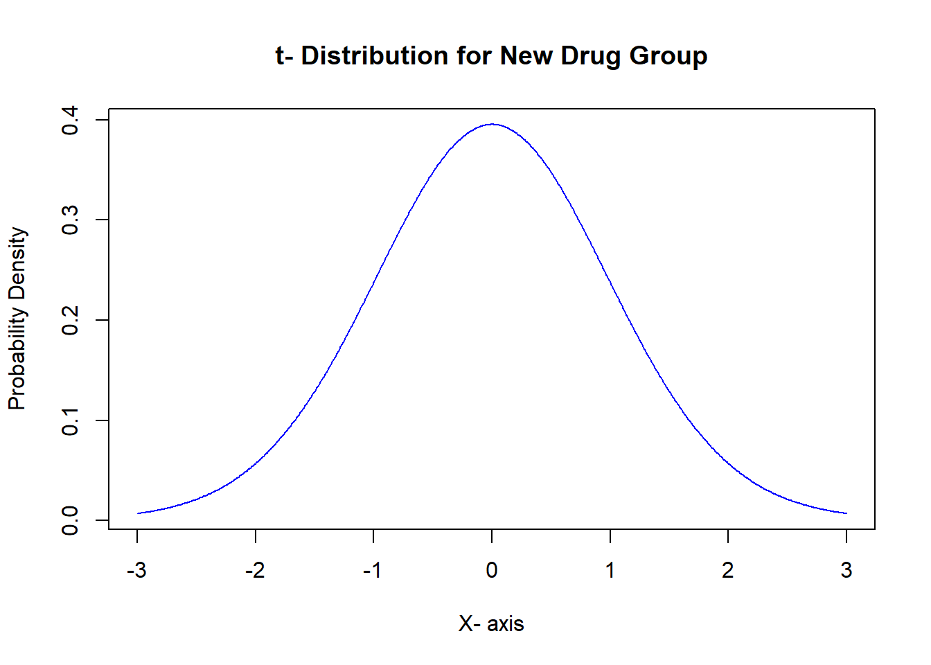 The t- statistic in a t- test helps you decide whether to reject the null hypothesis (H0) in favor of the alternative hypothesis (Ha) or not. It does this by quantifying how many standard errors the sample statistic (mean) is away from the hypothesized population parameter (mean under H0).
Here’s how the t- statistic helps you make decisions in a t- test:
Magnitude of the t- Statistic:
The t- statistic is a measure of how extreme your sample result is compared to what you would expect if the null hypothesis were true. A larger absolute t- statistic indicates a greater difference between the sample statistic and the hypothesized population parameter.
Degrees of Freedom (df):
The degrees of freedom associated with the t- distribution depend on the sample size. In a one- sample t- test, df equals the sample size minus 1 (df = n - 1).
T- Distribution:
The t- statistic follows a t- distribution, which is a bell- shaped distribution similar to the normal distribution but with heavier tails. The shape of the t- distribution depends on the degrees of freedom.
P- Value:
The t- statistic, along with the degrees of freedom, is used to calculate the p- value. The p- value tells you the probability of observing a result as extreme as, or more extreme than, the one obtained if the null hypothesis were true. Comparison to Significance Level (Alpha): You compare the p- value to your chosen significance level (alpha) to make a decision. Common alpha values are 0.05 (5%) or 0.01 (1%).
Now, the decision- making process based on the t- statistic and p- value:
- If the absolute value of the t- statistic is large, and the p- value is small (typically less than your chosen alpha), it suggests that your sample result is significantly different from what you would expect under the null hypothesis. In this case, you would reject the null hypothesis (H0) in favor of the alternative hypothesis (Ha).
- If the absolute value of the t- statistic is small, or if the p- value is large (greater than alpha), it suggests that your sample result is not significantly different from what you would expect under the null hypothesis. In this case, you would fail to reject the null hypothesis.
So, the t- statistic helps you decide whether the observed difference in your sample is statistically significant or whether it could have occurred due to random variation, as assumed by the null hypothesis.
7.2 Chi- Squared Tests for Categorical Data:
Chi- squared tests are used when you want to assess the association between two categorical variables or determine if observed categorical data differs significantly from expected values. There are two main types: the chi- squared test for independence and the chi- squared goodness- of- fit test.
Assumptions of Chi- square test:
Independence of Observations: The observations in the contingency table must be independent. This means that the data should not come from a paired or matched design. If there is a natural pairing or dependency in the data, a different statistical test may be more appropriate.
Random Sampling: The data should come from a random sample or a random sampling process. Non- random sampling may introduce bias and affect the validity of the test results.
Categorical Data: The chi- square test is designed for analyzing categorical data, where variables are divided into categories or groups. It is not suitable for continuous data.
Expected Frequencies: Each cell in the contingency table (cross- tabulation) should have an expected frequency greater than 5. In cases where expected frequencies are less than 5, you may need to consider alternatives like Fisher’s Exact Test or apply corrections, such as the Yates’ correction for continuity.
No Cell with Zero Frequency: There should be no cell in the contingency table with a frequency of zero. A cell with zero frequency means that a particular combination of categories did not occur in the data, making it impossible to calculate a chi- square statistic.
Sufficient Sample Size: In practice, a larger sample size tends to yield more reliable results. If the sample size is extremely small, even if the expected frequencies are greater than 5, the chi- square test may not be very informative or powerful.
Mutually Exclusive Categories: Categories within each variable should be mutually exclusive. Each observation should belong to only one category for each variable in the contingency table.
No Missing Data: The data used for the chi- square test should not have missing values for the variables under consideration. Missing data can lead to biased results.
Example:
To assess if gender is independent of job satisfaction, you collect data on both variables and use a chi- squared test for independence. If the p- value is low, you can conclude that there’s a significant relationship between gender and job satisfaction.
# Create a more complex sample dataset
set.seed(123)
gender <-  sample(c("Male", "Female", "Non- binary"), 100, replace = TRUE)
job_satisfaction <-  sample(c("Satisfied", "Dissatisfied", "Neutral"), 100, replace = TRUE)

# Create a data frame
data <-  data.frame(Gender = gender, JobSatisfaction = job_satisfaction)

# Create a contingency table
contingency_table <-  table(data$Gender, data$JobSatisfaction)

# Perform a chi- squared test for independence
chi_result <-  chisq.test(contingency_table)

# Print the test result
print(chi_result)
##
## Pearson's Chi-squared test
##
## data: contingency_table
## X-squared = 5.2, df = 4, p-value = 0.3# Visualize the contingency table
library(ggplot2)
ggplot(data, aes(x = Gender, fill = JobSatisfaction)) +
geom_bar(position = "fill") +
labs(title = "Gender vs. Job Satisfaction", x = "Gender", y = "Proportion") +
scale_fill_manual(values = c("Satisfied" = "green", "Dissatisfied" = "red", "Neutral" = "blue"))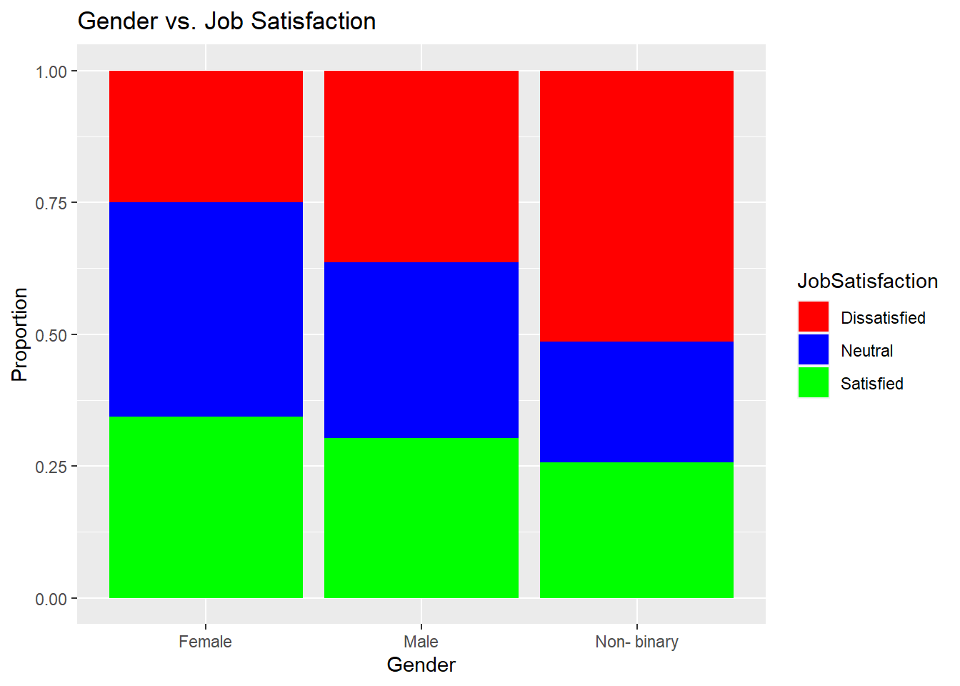 > The p- value is 0.2671 and is greater than the alpha so we can say that there isn’t a significant relationship between gender and job satisfaction, indicating that these variables are independent.
7.3 Interpreting p- Values:
A p- value is a crucial output in hypothesis testing. It represents the probability of obtaining the observed results (or more extreme) under the assumption that the null hypothesis is true. A smaller p- value suggests stronger evidence against the null hypothesis.
Example:
After performing a t- test on two groups of students’ test scores, you obtain a p- value of 0.03. If you set a significance level (alpha) of 0.05, the p- value is less than alpha, indicating that you can reject the null hypothesis and conclude that there’s a significant difference in test scores between the groups.
7.4 Fisher’s Exact Test:
Fisher’s Exact Test is a statistical method used to analyze the association between two categorical variables when sample sizes are small or when the assumptions of the chi- squared test are not met. It’s particularly useful when dealing with 2x2 contingency tables.
Assumptions:
Independence of Observations: Similar to the chi- square test, the observations in the contingency table for Fisher’s Exact Test should be independent. This means that the data should not come from a paired or matched design, and the observations should be unrelated to each other.
Categorical Data: Fisher’s Exact Test is designed for analyzing categorical data, where variables are divided into categories or groups. It is not suitable for continuous data.
Small Sample Size: Fisher’s Exact Test is particularly useful when dealing with small sample sizes. However, it can become computationally intensive for very large datasets, so it may not be the best choice in such cases.
Cell Frequencies: There should be no cell in the contingency table with a frequency of zero. In other words, all cells in the table should have at least one observation. The test is based on the hypergeometric distribution, and zero frequencies would result in division by zero in the calculation.
Unordered Categories: Unlike some chi- square tests that assume ordered categories (e.g., ordinal data), Fisher’s Exact Test does not require categories to be ordered. It can be applied to unordered categorical variables.
Exact Test: As the name suggests, Fisher’s Exact Test calculates exact probabilities based on the hypergeometric distribution. Therefore, it does not rely on large- sample approximations, making it suitable for small datasets.
Two- Sided or One- Sided Test: Fisher’s Exact Test can be performed as a two- sided test (to detect any association) or as a one- sided test (to detect a specific direction of association).
No Assumption of Homogeneity of Variance: Unlike some parametric tests, Fisher’s Exact Test does not assume homogeneity of variance between groups.
No Assumption of Normally Distributed Data: Fisher’s Exact Test is not based on the assumption of normally distributed data, making it robust to non- normally distributed data.
In summary, Fisher’s Exact Test is a valuable tool when dealing with small categorical datasets and is less sensitive to certain assumptions compared to chi- square tests. Example:
Imagine you’re studying the effectiveness of two different treatments (A and B) for a rare medical condition, and you have a small sample of patients. You create a 2x2 table with the number of patients who improved and those who didn’t for each treatment group. Fisher’s Exact Test can help determine if there’s a significant difference in treatment effectiveness, even with limited data.
Fisher’s Exact Test provides a p- value that, when compared to a chosen significance level (e.g., 0.05), allows you to decide whether the observed associations are statistically significant or likely due to chance.
# Create a 2x2 contingency table for treatment effectiveness (larger sample, more variations)
treatment_data <-  matrix(c(50, 50, 30, 70), nrow = 2,
                         dimnames = list(c("Treatment A", "Treatment B"),
                                         c("Improved", "Not Improved")))

# Perform Fisher's Exact Test
fisher_result <-  fisher.test(treatment_data)

# Print the test result
print(fisher_result)
##
## Fisher's Exact Test for Count Data
##
## data: treatment_data
## p-value = 0.006
## alternative hypothesis: true odds ratio is not equal to 1
## 95 percent confidence interval:
## 1.256 4.352
## sample estimates:
## odds ratio
## 2.323# Create a bar plot to visualize the data
library(ggplot2)
treatment_data_df <- as.data.frame(treatment_data)
treatment_data_df$Treatment <- row.names(treatment_data_df)
treatment_data_long <- tidyr::gather(treatment_data_df, key = "Outcome", value = "Count", - Treatment)
ggplot(treatment_data_long, aes(x = Treatment, y = Count, fill = Outcome)) +
geom_bar(stat = "identity", position = "dodge") +
labs(title = "Treatment Effectiveness", x = "Treatment", y = "Count") +
scale_fill_manual(values = c("Improved" = "green", "Not Improved" = "red"))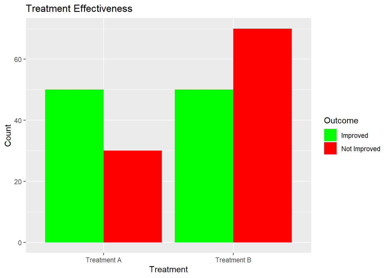 > As the p- value is small (typically less than your chosen significance level, e.g., 0.05), we can conclude that there’s a significant difference in treatment effectiveness between the two groups. This indicates that one treatment is more effective than the other, even with limited data.
Understanding these concepts is essential for making informed decisions based on data and drawing reliable conclusions in various fields, from medicine to social sciences.