Session-8 Case Study : The Deans Dilemma
Jain University’s Business School’s Dean, Easwaran lyer, needed to figure out some suitable parameters for the selection of students who were ideal for the Master of Business Administration (MBA) program. The University had around 400 seats for the MBA program and every year it received a lot of applications from all over the India. Over the years, it had been increasing the number of applications. In order to attract the right set of students to the MBA program, placement performance was very crucial in India. However, over 180 Business Schools were closed down in 2012 in different cities of the country, including Bangalore, Ahmedabad, Delhi, Mumbai, Dehradun, Kolkata, and Lucknow, which reflected various causes for their closure such as lack of expertise by the institute in promoting their students to play a major role in the field.
The Dean himself decided to participate in the screening process of the candidate’s application that either to be selected or rejected, along with his admission committee team from the start of the admission season that stretched to around 4 months from April to July. However, the management had no criteria of putting fine on the selection of non-placeable student, but it would ultimately affect the ranking of Jain University. The higher the number of wrong selections by the committee would cause the reduction in the average salary. Along with this, there was also a probability of rejecting a potential candidate. The challenge for Easwaran lyer was not only to increase the students in the batch, but also to ensure the admission of ideal students. He believed that to combat this challenge.
So how can you help the Dean in this challenge? Let’s analyse the case together.
Challenges
Challenges The key points and dilemmas in this scenario include:
High Volume of Applications: The MBA program at Jain University’s Business School receives a large number of applications from all over India, and this number has been increasing over the years.
Importance of Placement Performance: In the Indian context, placement performance is a critical factor for business schools. Attracting the right set of students who can secure good job placements upon graduation is essential.
Closure of Other Business Schools: The case mentions that numerous business schools in various cities across India had closed down in the past due to reasons such as inadequate student placements. This reflects the competitive landscape and the need for effective student placement strategies.
Dean’s Involvement in Admission Process: Dean Easwaran Iyer decides to actively participate in the screening process of MBA program applicants. This suggests his dedication to ensuring the selection of the right candidates for the program.
Lack of Criteria for Rejecting Students: While there is no clear criteria for rejecting students, making incorrect selections could have negative consequences for the university, including potential damage to its ranking and the average salary of graduates.
Balancing Quantity and Quality: Dean Iyer faces the challenge of not only increasing the number of students in the MBA program but also ensuring that the admitted students are the right fit for the program and have good job placement prospects.
Importance of Ideal Students: The Dean believes that admitting ideal students is essential to overcoming the challenges faced by the university in terms of student placements and maintaining its reputation.
The case study presents a common dilemma faced by academic institutions, particularly business schools, in ensuring that the students they admit are well-suited for their programs and will contribute positively to the institution’s reputation and performance metrics, including placement statistics. It highlights the importance of strategic admissions decisions in the context of higher education. Dean Iyer’s challenge is to strike a balance between quantity and quality while addressing the competitive dynamics of the Indian MBA education market.
Reading the Dean’s Dilemma case study dataset into a data frame for futher investigation and insights.
##   SlNo Gender Gender.B Percent_SSC Board_SSC
## 1    1      M        0       62.00    Others
## 2    2      M        0       76.33      ICSE
## 3    3      M        0       72.00    Others
## 4    4      M        0       60.00      CBSE
## 5    5      M        0       61.00      CBSE
##   Board_CBSE Board_ICSE Percent_HSC Board_HSC
## 1          0          0       88.00    Others
## 2          0          1       75.33    Others
## 3          0          0       78.00    Others
## 4          1          0       63.00      CBSE
## 5          1          0       55.00       ISC
##   Stream_HSC Percent_Degree         Course_Degree
## 1   Commerce          52.00               Science
## 2    Science          75.48 Computer Applications
## 3   Commerce          66.63           Engineering
## 4       Arts          58.00            Management
## 5    Science          54.00           Engineering
##   Degree_Engg Experience_Yrs Entrance_Test S.TEST
## 1           0              0           MAT      1
## 2           0              1           MAT      1
## 3           1              0          None      0
## 4           0              0           MAT      1
## 5           1              1           MAT      1
##   Percentile_ET S.TEST.SCORE Percent_MBA
## 1          55.0         55.0       58.80
## 2          86.5         86.5       66.28
## 3           0.0          0.0       52.91
## 4          75.0         75.0       57.80
## 5          66.0         66.0       59.43
##    Specialization_MBA Marks_Communication
## 1      Marketing & HR                  50
## 2 Marketing & Finance                  69
## 3 Marketing & Finance                  50
## 4 Marketing & Finance                  54
## 5      Marketing & HR                  52
##   Marks_Projectwork Marks_BOCA Placement Placement_B
## 1                65         74    Placed           1
## 2                70         75    Placed           1
## 3                61         59    Placed           1
## 4                66         62    Placed           1
## 5                65         67    Placed           1
##   Salary
## 1 270000
## 2 200000
## 3 240000
## 4 250000
## 5 180000Now having a further look into the Dataset by calculating the summary statistics for important variables.
##    Min. 1st Qu.  Median    Mean 3rd Qu.    Max.
## 37.0 56.0 64.5 64.7 74.0 87.2## Min. 1st Qu. Median Mean 3rd Qu. Max.
## 40.0 54.0 63.0 63.8 72.0 94.7## Min. 1st Qu. Median Mean 3rd Qu. Max.
## 35.0 57.5 63.0 63.0 69.0 89.0## vars n mean sd median trimmed mad min
## X1 1 391 219078 138312 240000 217012 88956 0
## max range skew kurtosis se
## X1 940000 940000 0.24 1.74 6995lets use R to calculate the median salary of all the students in the data sample
## [1] 240000Use R to calculate the percentage of students who were placed, correct to 2 decimal places.
##
## Not Placed     Placed
## 20.2 79.8## Length Class Mode
## 391 character character## [1] 79.8Lets use R to create a dataframe called placed, that contains a subset of only those students who were successfully placed.
newdata <- subset(deans_Dilema_df,Placement_B=='1',select=c(SlNo,Gender,Percent_SSC,
Percent_HSC,S.TEST.SCORE,Percent_MBA,Placement,Placement_B,Specialization_MBA,Salary))
head(newdata)
## SlNo Gender Percent_SSC Percent_HSC S.TEST.SCORE
## 1 1 M 62.00 88.00 55.0
## 2 2 M 76.33 75.33 86.5
## 3 3 M 72.00 78.00 0.0
## 4 4 M 60.00 63.00 75.0
## 5 5 M 61.00 55.00 66.0
## 6 6 M 55.00 64.00 0.0
## Percent_MBA Placement Placement_B
## 1 58.80 Placed 1
## 2 66.28 Placed 1
## 3 52.91 Placed 1
## 4 57.80 Placed 1
## 5 59.43 Placed 1
## 6 56.81 Placed 1
## Specialization_MBA Salary
## 1 Marketing & HR 270000
## 2 Marketing & Finance 200000
## 3 Marketing & Finance 240000
## 4 Marketing & Finance 250000
## 5 Marketing & HR 180000
## 6 Marketing & Finance 300000Lets use R to find the median salary of students who were placed.
## [1] 260000Lets use R to create a table showing the mean salary of males and females, who were placed.
##   Gender      x
## 1      F 253068
## 2      M 284242
Lets use R to generate the following histogram showing a breakup of the MBA performance of the students who were placed
hist(newdata$Percent_MBA,xlim=c(50,80),ylim=c(0,150),xlab="MBAPercentage",ylab="Count",breaks=3,main="MBA Performance of placed students",col=c("lightblue"))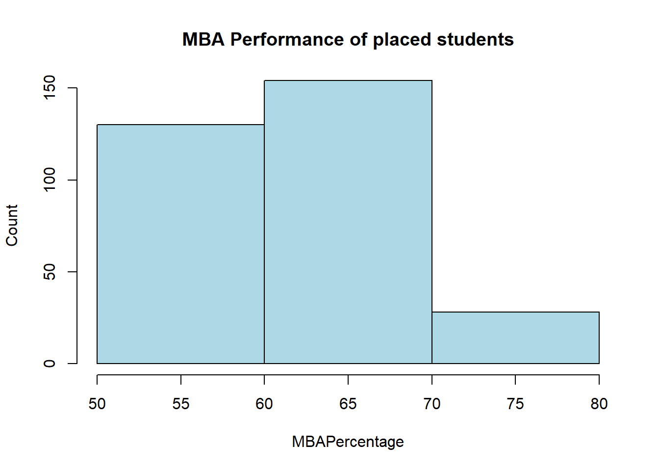
Lets create a dataframe called notplaced, that contains a subset of only those students who were NOT placed after their MBA.
notplaced <- subset(deans_Dilema_df,Placement_B=='0',select=c(SlNo,Gender,Percent_SSC,
Percent_HSC,S.TEST.SCORE,Percent_MBA,Placement,Placement_B,Specialization_MBA,Salary))
head(notplaced)
## SlNo Gender Percent_SSC Percent_HSC S.TEST.SCORE
## 11 11 F 79.60 87.0 98.69
## 16 16 F 49.00 52.2 74.28
## 20 20 M 66.00 46.0 0.00
## 40 40 F 60.00 75.0 60.00
## 42 42 F 40.00 40.0 49.00
## 43 43 M 77.12 85.0 35.00
## Percent_MBA Placement Placement_B
## 11 69.78 Not Placed 0
## 16 53.29 Not Placed 0
## 20 54.65 Not Placed 0
## 40 67.28 Not Placed 0
## 42 51.75 Not Placed 0
## 43 56.34 Not Placed 0
## Specialization_MBA Salary
## 11 Marketing & HR 0
## 16 Marketing & Finance 0
## 20 Marketing & Finance 0
## 40 Marketing & Finance 0
## 42 Marketing & Finance 0
## 43 Marketing & IB 0Draw two histograms side-by-side, visually comparing the MBA performance of Placed and Not Placed students, as follows:
par(mfrow=c(1,2))
hist(newdata$Percent_MBA,xlim=c(50,80),ylim=c(0,150),xlab="MBAPercentage",
     ylab="Count",
     breaks=3,
     main="MBA Performance of placed students",
     col=c("lightblue"))
hist(notplaced$Percent_MBA,xlim=c(50,80),ylim=c(0,150),xlab="MBAPercentage",
     ylab="Count",
     breaks=3,
     main="MBA Performance of placed students",
     col=c("lightblue"))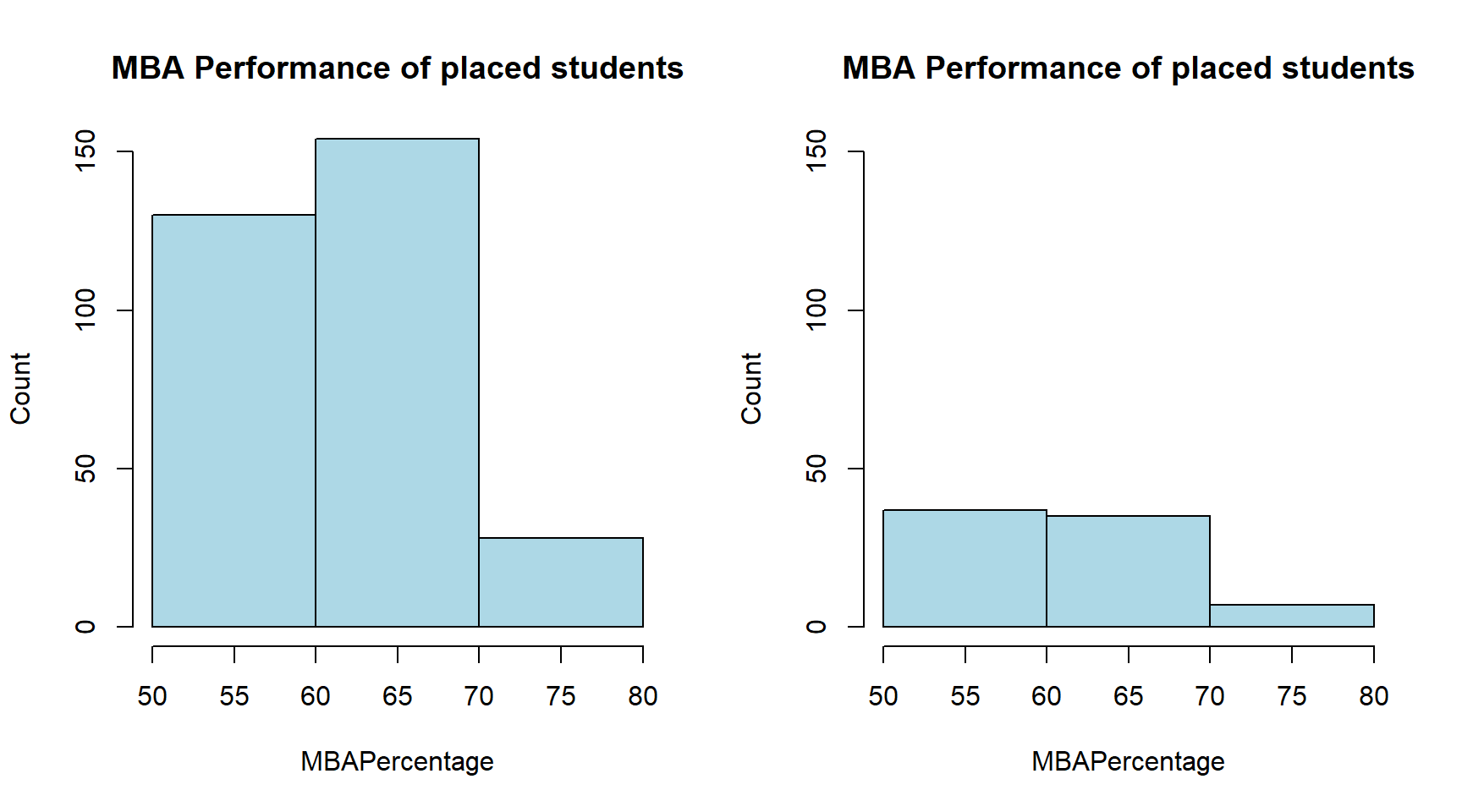
Lets use R to draw two boxplots, one below the other, comparing the distribution of salaries of males and females who were placed, as follows:
boxplot( Salary ~ Gender, data= newdata,horizontal=TRUE,yaxt="n",
        xlab="Salary",ylab="Gender",
        main="Comparison of Salaries of Male and Females")
        axis(side=2,at=c(1,2),labels=c("Females","Males"))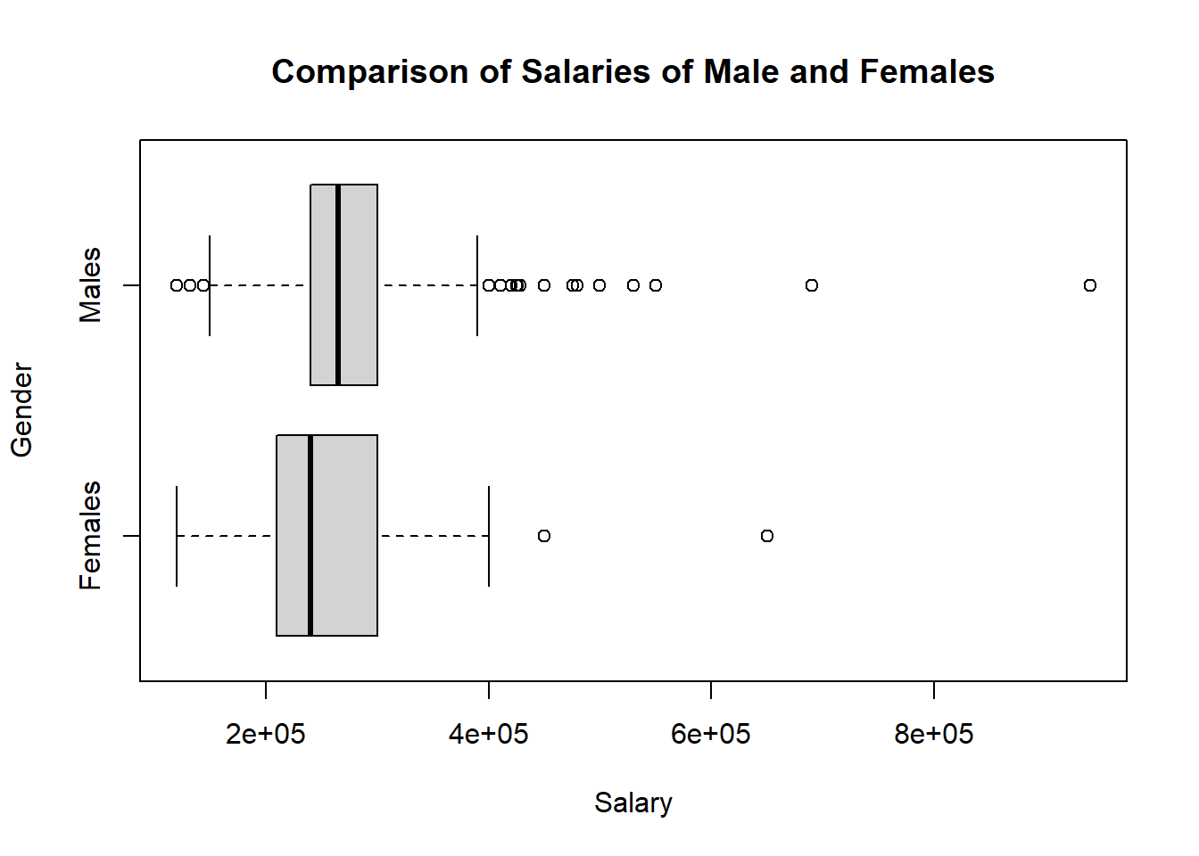
Lets create a dataframe called placedET, representing students who were placed after the MBA and who also gave some MBA entrance test before admission into the MBA program.
placedET <-  subset(deans_Dilema_df,Placement_B=='1' & S.TEST=='1',select=c(SlNo,Gender,Percent_SSC,
Percent_HSC,S.TEST.SCORE,Percent_MBA,Percentile_ET,Placement,Placement_B,Specialization_MBA,Salary))
head(placedET)
## SlNo Gender Percent_SSC Percent_HSC S.TEST.SCORE
## 1 1 M 62.00 88.00 55.00
## 2 2 M 76.33 75.33 86.50
## 4 4 M 60.00 63.00 75.00
## 5 5 M 61.00 55.00 66.00
## 8 8 M 68.00 77.00 43.12
## 9 9 M 82.80 70.60 96.80
## Percent_MBA Percentile_ET Placement Placement_B
## 1 58.80 55.00 Placed 1
## 2 66.28 86.50 Placed 1
## 4 57.80 75.00 Placed 1
## 5 59.43 66.00 Placed 1
## 8 57.23 43.12 Placed 1
## 9 55.50 96.80 Placed 1
## Specialization_MBA Salary
## 1 Marketing & HR 270000
## 2 Marketing & Finance 200000
## 4 Marketing & Finance 250000
## 5 Marketing & HR 180000
## 8 Marketing & Finance 235000
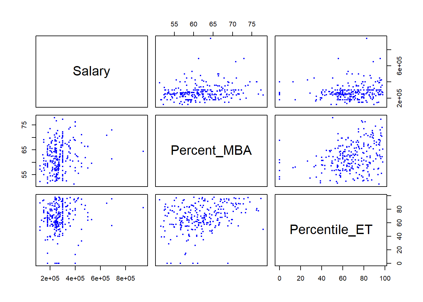
## 9 Marketing & Finance 425000Drawing a Scatter Plot Matrix for 3 variables – {Salary, Percent_MBA, Percentile_ET} using the dataframe placedET.
pairs(placedET[, c("Salary", "Percent_MBA", "Percentile_ET")],
      cex = 0.6,  # Set character size
      pch = 20,   # Set point type (optional)
      col = "blue"  # Set point color (optional)
)